Smarter, Not Harder: How actuaries automate work on GLMs using AI


Introduction
As discussed in the previous article, the process of manually creating a GLM (Generalised Linear Models) model is extremely time-consuming, particularly when dealing with numerous variables for testing and variables that possess multiple categories. Insurance companies are now accumulating vast amounts of data due to the inclusion of new data sources such as weather data, police data, telematics data, and other such sources.
Manually selecting features or combining related categories can be highly labour-intensive and error prone. In addition, the manual creation of a GLM model requires the numerous actuaries and pricing analysts, resulting in substantial expenses for insurance companies. Moreover, the process of creating a model can take several weeks or even months to complete, further increasing the time and financial costs.
The key to addressing the previously mentioned difficulties is the integration of AI-assisted functionalities in the process of building GLM models. AI can improve various activities, such as:
- feature selection,
- binning and mapping variables,
- detecting interaction,
- automated discovery of microsegments.
The incorporation of these functionalities not only results in considerable time savings, but it also enhances the overall quality of the models, ultimately leading to cost savings.
According to data provided by Mckinsey [1], the loss ratio of new business can be reduced by over 4 percentage points, and for renewals, it can be reduced by 1.3 percentage points using AI-based solution.
Feature selection
There are several statistical methods that can prove useful in feature selection and enable us to assess the degree to which a given variable impacts our target. This can allow us to discard a sizeable proportion of irrelevant variables at the outset, thereby saving considerable time.
Outlined below are several methods that you may consider using to select variables:
- Information Value,
- Gini score,
- GBM (Gradient Boosting Machine) importance.
Information Values
Information Value (IV) technique is widely used in statistical analysis to rank variables based on their importance. Although it is typically applied to logistic regression and categorical variables, it can be used with all GLM models and continuous variables.
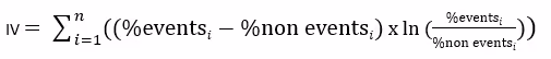
Information values for binary target are calculated by summing up the differences between the percentage of events and non-events for each category or bin of a variable, multiplied by the natural logarithm of the ratio between the percentage of events and non-events.
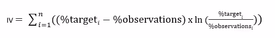
When calculating the IV for a continuous target variable, the process is slightly different. The IV is determined by summing the differences between the percentage of target and observations for each category or bin of a variable. This sum is then multiplied by the natural logarithm of the ratio between the percentage of target and observations.
One key factor that influences the IV result is the appropriate selection of bins or mapping of categorical variables. If a category has a very small percentage in the variable, but the target for that category is significant, it can lead to a large IV result and the variable being deemed significant. As such, it is crucial to ensure that the bins have the correct proportion of the dataset and are selected based on the target. This ensures that the IV method provides accurate results and allows us to identify the most important variables for our analysis.
You can read more about this method here [2].
Gini score
The Gini score is a widely used method in the insurance industry to evaluate the ability of a model to differentiate between clients. However, it is not limited to this specific use case and can also be applied to a single variable to assess its ability to distinguish between different values or categories. By computing the Gini score of a variable, we can determine the degree of differentiation it provides and evaluate its potential usefulness as a feature in our model. To use this technique, categorical variables should be mapped, and continuous variables should be binned, as in the process of calculating Information Values. Once the variables have been prepared, the Gini score can be computed to assess how strongly each variable differentiates our set.
Gini score for a variable is calculated as follows:
- Sort categories/bins by target mean in ascending order.
- Calculate cumulative proportion of the target.
- Calculate cumulative proportion of observations.
- Measure the area between the curve formed from the points calculated above and the diagonal line.
Variables with higher Gini scores indicate a stronger differentiation, while those with a score close to 0 have no effect on our target.
One of the benefits of using the Gini score for feature selection is its efficiency in computation and ease of interpretation.
GBM importance
Gradient Boosting Machine (GBM) is a powerful machine learning algorithm that has gained widespread popularity in recent years due to its ability to handle complex datasets and produce accurate predictions. In addition to its high predictive power, GBM also offers a useful feature selection method, which can help identify the most important input features for a given problem.
There are two main types of GBM importance measures: "split" and "gain".
The "split" importance measure is based on the number of times a feature is used to split the data during the construction of the decision trees in the GBM model. Features that are used more frequently for splitting are regarded as more crucial.
The "gain" importance measure is based on the total reduction in the loss function (e.g., mean squared error or binary cross-entropy) achieved by using a particular feature to split the data. Features that result in greater reductions in loss are deemed to hold greater significance.
Compared to the two previously mentioned methods, this method involves building a separate model specifically to calculate the importance of variables. Therefore, the variables identified as important in this model may not necessarily be as significant in the GLM model. Furthermore, parameters of the GBM model can significantly affect the result of feature importance.
Optimal binning and mapping
Although it is possible to manually create bins for continuous variables or mapping categorical variables, this can be a time-consuming and inefficient process. Additionally, it can be difficult to determine whether the chosen bins or mappings are optimal for our model. To address this issue, we can use decision trees to automatically identify the best splits or mappings for our variables.
The basic idea behind optimal binning is to find the best possible grouping of values for a given variable, either categorical or continuous. This grouping aims to maximize the difference in target variable values between adjacent bins while minimizing the variance within each bin.
For numerical variables this is achieved by calculating the optimal cut point for each pair of adjacent bins, which divides the range of values between the two bins into two groups with the minimum difference in their mean target variable values. This process is repeated iteratively until the optimal cut points are found for all adjacent pairs of bins, resulting in the most effective binning scheme for the given variable.
For categorical variables, the optimal binning process is slightly different. The optimal binning algorithm starts by treating each unique category in the variable as an individual bin. Then, it iteratively merges adjacent bins until no further merging improves the chosen criteria.
Ensuring an appropriate number of observations within each bin is crucial to avoid issues such as overfitting or insufficient differentiation between bins. If the number of observations in a bin is too small, it can lead to overfitting and instability in the model. On the other hand, if there are too many observations in a bin, the differentiation between bins may not be significant enough, negatively impacting the model's performance.
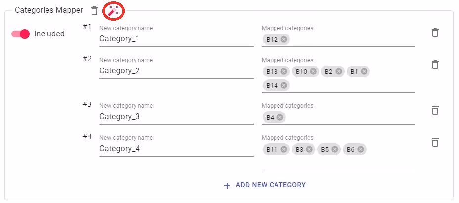
Quantee platform allows the Users to easily find the optimal bins and mappings. Just use the magic wand!

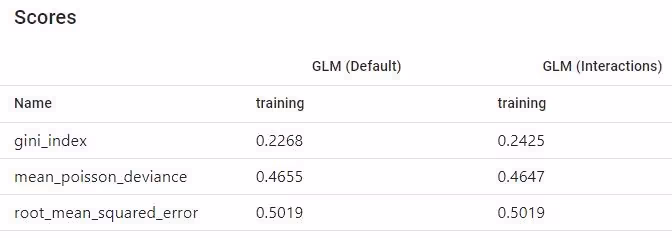
Interactions
When two explanatory variables have an interaction effect, the prediction cannot be simply expressed as a sum of the effects of the variables, since the impact of one variable is dependent on the value of the other. Identifying these interactions can be challenging as the number of variables and combinations increases.
Friedman's H-statistic
The Friedman's H-statistic approach can help in such situations as it measures how much of the variation of the prediction depends on the interaction of the features. The calculation of Friedman's H-statistic involves determining the difference between a two-way partial dependence function and the sum of two one-way partial dependence functions for each of the two features involved in the interaction.
However, this method has a significant drawback: it is computationally expensive, and therefore takes a considerable amount of time to compute.
One-way chart
A One-way chart with segmentation is a straightforward and effective method to identify interactions between variables. By using this chart, we can not only determine which variables interact but also pinpoint the exact values at which the interaction occurs.
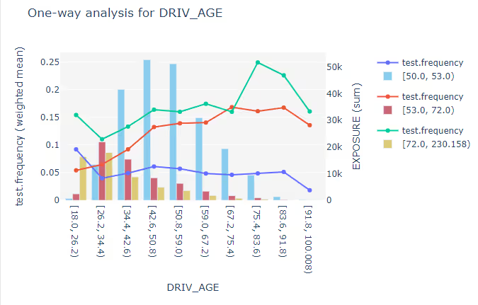
Based on the chart, we can conclude that above the risk class 53, driver age has a strong impact on the frequency.
Microsegments
Micro-segmentation is a more detailed and specific form of segmentation, where customers are divided into smaller, non-overlapping groups based on their unique characteristics and behaviours. By analysing these microsegments, businesses can gain deeper insights into the needs and preferences of their target customers, and tailor their marketing strategies, product offerings, and services accordingly. This can lead to more effective customer engagement and higher levels of customer satisfaction, as well as increased sales and revenue for the business.
Conclusion
Above, we have outlined several statistical methods that can enhance, accelerate, and streamline the modelling process. Each of the feature selection methods: IV, the Gini score, and GBM importance has its own set of advantages and disadvantages. While IV and the Gini score are straightforward to compute and understand and demonstrate a clear connection between the variable and the target, they are heavily reliant on the proper binning and mapping. On the other hand, with GBM importance the challenge is to select the appropriate model parameters to prevent overfitting or underfitting. Ultimately, selecting the appropriate method is dependent on the problem and the data at hand.
Utilizing AI-assisted functionalities such as optimal binning selection or interaction detection not only results in significant time savings but also enhances the accuracy and efficiency of our model.
%25204x.avif)
If you are looking for a tool that can assist you in the modelling process, please do not hesitate to contact us.
References
[2] https://www.lexjansen.com/sesug/2014/SD-20.pdf
[3] https://christophm.github.io/interpretable-ml-book/interaction.html