Insurance Pricing with Interpretable Machine Learning

An insurance applicant may wonder how the premium for a motor policy had been calculated. The decision must take several different factors into account, such as driving record, horsepower or driver’s age, all provided by the intended policyowner. However, the exact inner workings of the pricing process are usually a black-box to the applicant. Similarly to credit approval process in the banking sector, it is beneficial that insurers are able to explain the decision to a particular policy applicant. Fortunately, data scientists are developing a new exciting field - Explainable Artificial Intelligence - which can be efficiently used to accomplish the task. This article aims to present basic pricing techniques, explain more sophisticated methods such as machine learning algorithms and finally show how Explainable AI can be used by insurance management and actuaries to disrupt current pricing techniques.

Pricing Basics

Policy pricing process aims to incorporate all available information, use actuarial model and return a fair price, increasing with the level of risk covered by the insurer. When the market situation and competition is considered, a distinction is usually drawn: calculating a fair premium using actuarial techniques is often referred to as costing, while pricing itself means the final commercial decision, partially based on results delivered by actuaries. In general, the two might not comply. All in all, according to Parodi pricing should be viewed as complex company-wide process, requiring several functions to cooperate.

A standard way to model losses in non-life insurance is to split them into claim frequency (claim counts) and severity (amounts of single claims), model those separately, and then combine using e.g. Monte Carlo methods. Here, for the sake of simplicity, we will focus on the first module. Poisson Generalized Linear Model (GLM) is what first comes to mind when trying to infer about count data. However, it enforces a rigid log-linear relationship between policyholder characteristics and prediction. One could introduce interactions between explanatory variables, and this is usually the way to go in actuarial departments, but model selection quickly becomes cumbersome with inflating feature space. Machine learning techniques enter the scene here, offering a universe of simple-to-use non-linear models. We will compare some standard model classes to demonstrate how more complexity allows us to capture the non-linear behaviour.

Case Study

For the practical part, we will use a motor third party liability insurance dataset prepared by Wuethrich and Buser for their comprehensive paper Data Analytics for Non-Life Insurance Pricing. It consists of 500 000 policies with the following characteristics:

• Car age 0 to 35, numeric,
• Driver age 18 to 90, numeric,
• Area A to F, ordinal, type of living area of the driver, from rural to large urban,
• Car brand 11 classes, categorical, B11 is the most powerful, eagerly chosen by young drivers,
• Population density 0 to 27 000, numeric,
• Fuel type Regular or Diesel, categorical,
• Horsepower 1 to 12, numeric,
• Canton 26 classes, categorical.

We drop the canton name variable, because it would blur the image due to its many categories. Area is ordinal and is recoded {A, …, B} -> {1, …, 6}. Number of claims per year per policyholder is what we are trying to predict. Models are trained on 400 000 training observations and compared using Poisson deviance loss on 100 000 test observations. We tried a standard GLM, LightGBM (a fast implementation of Gradient Boosting Machine, an ensemble of decision trees) and a simple feed-forward neural network, all with Poisson loss. The table below presents a comparison of the performance of three models measured by deviance on the test set - a standard metric used in actuarial pricing. The lower value of deviance, the higher quality of statistical model.

‍

‍

Both LightGBM and neural network outperform the GLM, with the former being the best. In general, multiple publications have proven machine learning techniques to work better than classical models, by a wide margin. So why are they not ubiquitous in actuarial modelling, despite their obvious advantage in predictive power? It is their lack of interpretability. This is particularly important to gain acceptance of financial supervision authorities or provide clients with the explanation they have the right to. GLMs are deemed interpretable because estimated model parameters have neat interpretations as factors which scale the output multiplicatively. However, the area of Interpretable Machine Learning or Explainable AI provides actuaries with various techniques which can help in explaining the predictions of arbitrarily complex, black-box models.

Interpretable Machine Learning

A good way to walk through explanations is to tell stories of artificial policyholders and describe their predictions with the use of explainers. We are operating in a Swiss setting, so let us introduce Ulrich, an entrepreneur from Zurich (population density 4 700, area code F) aged 25. He has a two-year-old car from brand B11, running on regular fuel, with 12 units of horsepower. For him, the three models returned the following predictions:

‍

‍

We can see that the GLM, being the worst fit, overstated Ulrich’s claim frequency. This would result in an unnecessarily high policy price. We would like to stress this point again: more accurate actuarial models yield fairer prices.

Before we proceed to explain Ulrich’s predictions, let us take a look at the global model characteristics. Firstly, we can examine which features have been important for generating the prediction. The approach we use here resembles the one used for random forests: an increase in loss after permutation of the variable of choice is investigated.

‍

‍

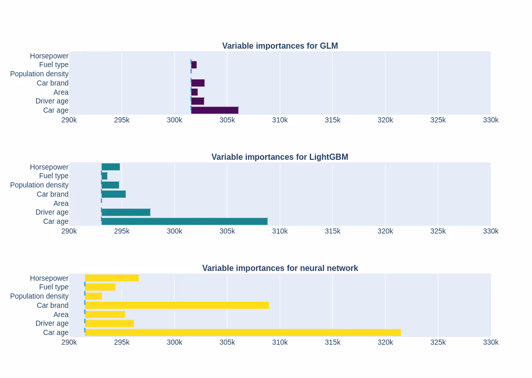
We can clearly see that car age and brand, as well as driver age, all play major roles. This is reasonable at an intuitive level. Considering claim frequency alone, we might have expected population density to be more important.

Now, let us see how the average model prediction changes with continuous variables. We will use Partial Dependency Plots, first introduced by Friedman in 1999.

‍

‍

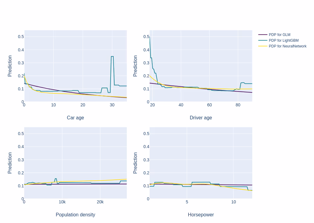
As we would expect, the GLM returns rigid, almost linear dependencies, which fail to capture more complex behaviour, e.g. for car age and driver age. LightGBM and neural network detected the significant increase in frequency for young ages. In addition, there is a jump for car age = 30 for the LightGBM PDP, but it can be explained with much higher mean frequency for car ages around 30 in the training sample.

Finally, a technique called BreakDown allows us to decompose a specific prediction into influences generated by each separate variable. It is the tool one would like to use to explain a decision to the customer. Be it pricing or credit scoring, it allows us to tell which variable influenced the final decision the most.

‍

‍

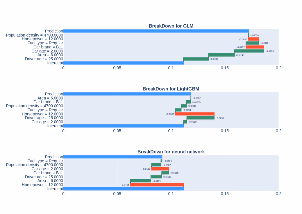
The attribution signs are broadly the same for all models, but different variables are stressed. The increased predicted frequency for an urban area, high population density and low age all are what we would expect. What the GLM failed to capture is the considerable negative effect of high horsepower detected by LightGBM and neural network. It might be so that people owning very powerful cars drive carefully or not too often.

Conclusions

Summarising, both insurance companies and their customers could benefit from the adoption of machine learning techniques. The actuaries and pricing departments are encouraged to minimize the black-box-ness of sophisticated algorithms with Explainable AI methods and visualizations. Using these algorithms to price Ulrich’s insurance would result in a lower price when compared with the GLM which failed to notice the risk lowering the effect of high horsepower of his car. On the other hand, more sophisticated models are better at detection of policy applicants with higher risk. Offering such people higher prices would help the insurer mitigate adverse selection. Using more accurate techniques in the competitive market is inevitable – but we can expect all of its participants to benefit.

‍